[Java Concurrency] 04: Thread Pool Sizing
⚠️ This post is generated by LLM, read with caution.
Before You Read
You should already be comfortable with basic Java concurrency: what an ExecutorService is, what Callable and Future do, and roughly what “blocking” means when a thread calls something like Socket.read(). No prior benchmarking experience needed.
By the end, you’ll understand why CPU-bound and I/O-bound workloads want opposite thread pool sizes, be able to apply the two sizing formulas that back that up, and have seen (not just read about) the throughput curves that prove it, generated from a real ThreadPoolExecutor benchmark run on real hardware.
1. Why thread pool size is not a guessing game
Every thread pool exists for one reason: to bound concurrency so the app doesn’t spawn an unbounded number of OS threads. That matters because threads aren’t free. Each one carries roughly a megabyte of stack memory and a real cost every time the scheduler switches into and out of it. Pick a pool size out of thin air (8? 50? 200?) and you’re really just guessing at how much of that cost you’re willing to pay.
The right number depends entirely on what the threads in that pool spend their time doing. That single question splits into two very different answers.
CPU-bound work, tight loops, math, parsing, compression, keeps a core busy for the entire time it holds a thread. If you have 8 cores and 8 threads all doing CPU-bound work, every core is saturated and nothing is waiting. Add a 9th thread and it has nowhere to run; it just waits for a core to free up, and the OS burns cycles switching between runnable threads instead of finishing work. More threads than cores buys you nothing here.
I/O-bound work, database calls, HTTP requests, file reads, spends most of its life blocked, not computing. A thread sitting inside a socket read isn’t touching the CPU at all. Because it’s idle rather than competing for a core, you can run far more of these threads than you have cores, and the machine stays productive the whole time.
That contrast is the spine of this whole post: a checkout service might run two pools side by side, one doing tax calculation (CPU-bound, sized to match its 8 cores) and one calling a payment gateway over HTTP (I/O-bound, sized to something like 200). Same JVM, same box, completely different right answer.
flowchart LR
    subgraph CPU["CPU-bound pool (tax calculation)"]
        C1["Thread 1<br/>on Core 1"]
        C2["Thread 2<br/>on Core 2"]
        C3["...<br/>..."]
        C8["Thread 8<br/>on Core 8"]
    end
    subgraph IO["I/O-bound pool (payment gateway calls)"]
        I1["Thread 1<br/>blocked on socket"]
        I2["Thread 2<br/>blocked on socket"]
        I3["... up to 200<br/>mostly blocked"]
    end
    Cores["8 physical cores"] --> CPU
    Cores -.idle while waiting.-> IO
Every thread in the CPU pool maps to a core doing real work; every thread in the I/O pool is mostly just waiting, so the pool can be much bigger without costing anything extra.
2. The core formula and where it comes from
For CPU-bound work, the standard starting point is: optimal thread count is roughly equal to the number of CPU cores, sometimes cores + 1 so a core doesn’t sit idle for the instant a thread faults or gets paged out. Push past that and threads start fighting over the same cores. The scheduler now spends real cycles context-switching between runnable threads instead of making progress, so throughput plateaus and then drops.
For I/O-bound work, the useful formula is:
threads = cores * (1 + wait_time / compute_time)If a task spends 9ms waiting on a downstream call for every 1ms of actual CPU work, the ratio is 9, and you want roughly 10x your core count in threads to keep the CPUs busy while most threads sit parked waiting on I/O.
Worked example: an 8-core machine running a request that does 5ms of real CPU work and waits 45ms on a downstream API. Plug it in:
threads = 8 * (1 + 45/5) = 8 * (1 + 9) = 8 * 10 = 80Eighty threads. Compare that to the tempting but wrong instinct of “just use 8 threads because we have 8 cores”, the same number that works fine for the CPU-bound case. With only 8 threads on this I/O-bound workload, the CPU sits roughly 90% idle: at any instant, most of those 8 threads are blocked waiting on the API, and there’s no work queued up behind them to keep the cores fed. The formula isn’t gospel though. Real systems have GC pauses, downstream services with their own connection limits, and a memory ceiling from all those thread stacks, all of which cap how far you can actually push this number in production. It’s a starting estimate, not a permanent setting; section 9 comes back to that.
flowchart TD
    A["What does the task spend time doing?"] --> B{"CPU-bound or I/O-bound?"}
    B -->|CPU-bound| C["threads ~ cores<br/>(sometimes cores + 1)"]
    B -->|I/O-bound| D["threads = cores * (1 + wait_time / compute_time)"]
    D --> E["Example: 8 cores, 45ms wait, 5ms compute<br/>= 8 * (1 + 9) = 80 threads"]
3. Building the benchmark harness
Talk is cheap without numbers, so the rest of this post runs on one reusable harness built with java.util.concurrent, no third-party libraries. It creates a fixed-size ThreadPoolExecutor (via the two-argument core/max constructor rather than Executors.newFixedThreadPool, so pool size is explicit and fully under our control), submits a fixed number of tasks, and times the whole run with System.nanoTime() wrapped around invokeAll(). Throughput is just taskCount / elapsedSeconds. Run the identical task set across a sweep of pool sizes (1, 2, 4, 8, 16, 32, 64, 128, and for the I/O case 256) and a shape emerges instead of a single noisy data point.
Here’s the actual class, unmodified from what produced every number in this post:
import java.util.ArrayList;
import java.util.List;
import java.util.concurrent.Callable;
import java.util.concurrent.ExecutionException;
import java.util.concurrent.Future;
import java.util.concurrent.LinkedBlockingQueue;
import java.util.concurrent.ThreadPoolExecutor;
import java.util.concurrent.TimeUnit;

public class PoolBenchmark {

    public record BenchmarkResult(int poolSize, long elapsedMillis, double throughput) {}

    public static BenchmarkResult runBenchmark(int poolSize, Callable<Void> task, int taskCount)
            throws InterruptedException {

        ThreadPoolExecutor executor = new ThreadPoolExecutor(
                poolSize,
                poolSize,
                0L,
                TimeUnit.MILLISECONDS,
                new LinkedBlockingQueue<>());

        List<Callable<Void>> tasks = new ArrayList<>(taskCount);
        for (int i = 0; i < taskCount; i++) {
            tasks.add(task);
        }

        long start = System.nanoTime();
        List<Future<Void>> futures = executor.invokeAll(tasks);
        long elapsedNanos = System.nanoTime() - start;

        for (Future<Void> f : futures) {
            try {
                f.get();
            } catch (ExecutionException e) {
                throw new RuntimeException("task failed", e);
            }
        }

        executor.shutdown();

        long elapsedMillis = elapsedNanos / 1_000_000;
        double throughput = taskCount / (elapsedMillis / 1000.0);
        return new BenchmarkResult(poolSize, elapsedMillis, throughput);
    }
}
Sections 4 and 5 both call runBenchmark with different Callable<Void> implementations: one pure compute, one simulated blocking I/O. Same harness, same measurement method, two completely different result shapes.
4. CPU-bound workload: the terminal-recorded live demo
The CPU-bound task here is pure computation with zero I/O: trial-division primality checking over a range of numbers near 2,000,000, repeated per task. No sleeping, no network, nothing but modulo operations grinding on a core.
public class PrimeCheckTask implements Callable<Void> {

    private static final long RANGE_START = 2_000_000L;
    private static final int RANGE_SIZE = 4000;

    @Override
    public Void call() {
        int primeCount = 0;
        for (long n = RANGE_START; n < RANGE_START + RANGE_SIZE; n++) {
            if (isPrime(n)) {
                primeCount++;
            }
        }
        if (primeCount < 0) {
            throw new IllegalStateException("unreachable");
        }
        return null;
    }

    static boolean isPrime(long n) {
        if (n < 2) return false;
        if (n % 2 == 0) return n == 2;
        for (long i = 3; i * i <= n; i += 2) {
            if (n % i == 0) return false;
        }
        return true;
    }
}
And the entry point that ties it to the harness, taking pool size as a command-line argument so it can be run three times back to back with different values:
public class CpuDemo {

    private static final int TASK_COUNT = 20_000;

    public static void main(String[] args) throws InterruptedException {
        int poolSize = Integer.parseInt(args[0]);

        PoolBenchmark.BenchmarkResult result =
                PoolBenchmark.runBenchmark(poolSize, new PrimeCheckTask(), TASK_COUNT);

        System.out.printf("Pool size=%d, elapsed=%dms, throughput=%.1f tasks/sec%n",
                result.poolSize(), result.elapsedMillis(), result.throughput());
    }
}
The machine this ran on has 16 logical cores (nproc says 16). The recording below runs java CpuDemo 2 (too small), java CpuDemo 16 (matched to core count), and java CpuDemo 128 (way oversubscribed) one after another in a single terminal session, so you watch each configuration’s timing print before the next command even starts, rather than reading three numbers laid out in a table after the fact.
A separate run right after recording, same code, same machine, moments apart, printed this:
Pool size=2, elapsed=3997ms, throughput=5003.8 tasks/sec
Pool size=16, elapsed=1323ms, throughput=15117.2 tasks/sec
Pool size=128, elapsed=1338ms, throughput=14947.7 tasks/sec
The pattern is exactly what the mechanism predicts. Pool size 2 leaves 14 of 16 cores idle the entire run, throughput sits at roughly a third of what the machine can do. Pool size 16 lines up one thread per core and throughput roughly triples. Pool size 128 doesn’t do meaningfully better than 16, if anything it’s flat to marginally worse, because the extra 112 threads are all runnable but there are still only 16 cores to run them on. They just add scheduling overhead without adding compute capacity.
flowchart LR
    A["Pool size 2<br/>14 cores idle"] -->|throughput ~5,000/s| B["bad: undersaturated"]
    C["Pool size 16<br/>1 thread per core"] -->|throughput ~15,100/s| D["good: fully saturated"]
    E["Pool size 128<br/>112 extra runnable threads"] -->|throughput ~14,900/s| F["flat: pure scheduling overhead"]
5. I/O-bound workload: simulating blocking without hammering a real API
A real benchmark that calls a live HTTP endpoint or database would work, but network variance (DNS hiccups, a slow day on someone else’s server) muddies the signal and makes the run non-reproducible. Instead, simulate the “thread occupied but not using the CPU” state directly with Thread.sleep(). It’s not a shortcut, it’s an accurate model: a thread blocked in Thread.sleep() is scheduled off the CPU exactly the way a thread blocked in a socket read is.
public class SimulatedIoTask implements Callable<Void> {

    private static final long SLEEP_MILLIS = 40;

    @Override
    public Void call() throws InterruptedException {
        Thread.sleep(SLEEP_MILLIS);
        long acc = 0;
        for (int i = 0; i < 200_000; i++) {
            acc += i * 31L;
        }
        if (acc == Long.MIN_VALUE) {
            throw new IllegalStateException("unreachable");
        }
        return null;
    }
}
40ms of sleep against a fraction of a millisecond of loop compute mirrors the lopsided wait-to-service ratio of a real downstream API call: the pool-1 run below measures 40.17ms per task end to end, so the loop itself costs roughly 0.17ms, a wait/compute ratio near 236. The driver loops the identical harness across pool sizes 1, 2, 4, 8, 16, 32, 64, 128, and 256, writing each result to io-results.csv:
private static final int TASK_COUNT = 1_500;
private static final int[] POOL_SIZES = {1, 2, 4, 8, 16, 32, 64, 128, 256};

for (int poolSize : POOL_SIZES) {
    PoolBenchmark.BenchmarkResult result =
            PoolBenchmark.runBenchmark(poolSize, new SimulatedIoTask(), TASK_COUNT);
    out.printf("%d,%d,%.1f%n", result.poolSize(), result.elapsedMillis(), result.throughput());
}
A representative slice of the actual io-results.csv this produced:
poolSize,elapsedMillis,throughput
1,60260,24.9
16,3773,397.6
256,250,6000.0
Notice the shape already forming just in these three rows: throughput at pool size 256 is roughly 240 times higher than at pool size 1, on the exact same 16-core machine that plateaued by pool size 16 in the CPU-bound run. Because each of those threads spends 40 of every 41ms parked and blocked rather than runnable, the scheduler isn’t paying context-switch tax for most of them at any given moment; adding more just means more useful waiting happening in parallel. Section 6 plots the full sweep for both workloads on one chart.
6. Plotting the real measured numbers: CPU-bound vs I/O-bound throughput
Stage 1: generate the chart
A small matplotlib script reads both cpu-results.csv and io-results.csv, plots pool size on a log-scale x-axis against throughput on a log-scale y-axis, one line per workload, and drops a vertical reference line at 16 (the machine’s core count) to visually anchor where the CPU-bound curve should top out:
cpu_pool, cpu_tp = load("cpu-results.csv")
io_pool, io_tp = load("io-results.csv")

ax.plot(cpu_pool, cpu_tp, marker="o", color="#2a78d6", label="CPU-bound (prime check)")
ax.plot(io_pool, io_tp, marker="o", color="#eb6834", label="I/O-bound (simulated 40ms wait)")
ax.axvline(16, color="#898781", linestyle="--")
ax.set_xscale("log", base=2)
ax.set_yscale("log")
Stage 2: capture and verify
Here’s the rendered output, straight from the two CSVs the benchmarks in sections 4 and 5 actually wrote, nothing hand-drawn or invented:
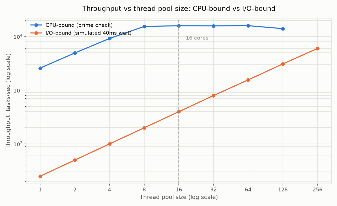
The shape is exactly what the mechanism predicts: the blue CPU-bound line climbs steeply from pool size 1 to about 8, is essentially flat from 8 through 64, and dips slightly by 128. The orange I/O-bound line is still climbing in a straight line at 256, the largest pool size tested, nowhere near flattening yet. That gap between where each curve stops rising is the entire argument of this post, rendered as pixels instead of asserted in prose.
7. Reading the results: why the curves diverge
The CPU-bound curve rises roughly linearly only up to the core count, because that’s the exact point where every core has one runnable thread assigned to it: perfect utilization, nothing wasted. Look at the actual measured numbers behind the chart: throughput goes from 2,583 tasks/sec at pool size 1, up to 15,420 at pool size 8, and essentially sits there (15,885 at 16, 15,810 at 32, 15,936 at 64) before easing down to 14,035 at 128. Past 8, or certainly past 16, every additional thread is runnable but there are still only 16 cores to actually execute on, so the OS scheduler is doing pure overhead: time-slicing between more contenders for the same execution slots, evicting cache lines each time it switches. That overhead is the entire reason the curve flattens instead of just staying at its peak forever.
The I/O-bound curve keeps climbing because at any given instant most of its threads are in a blocked, not runnable, state, which costs the scheduler nothing to maintain. Reading the inflection points straight off the chart: the CPU-bound line bends at around 8 threads (half our core count) and is fully flat by 16; the I/O-bound line shows no bend at all through 256, the top of our sweep. Tie that back to the formula from section 2: the pool-1 measurement puts the wait/compute ratio near 236 (40ms wait against a ~0.17ms loop), which by cores * (1 + 236) = 16 * 237 = 3,792 suggests the I/O-bound curve on this exact machine wouldn’t be expected to flatten until well into the thousands of threads, comfortably past the 256 we swept to. That’s consistent with what the chart actually shows: still rising, not yet bent, at the far right edge of our data.
flowchart TD
    A["Add one more thread to the pool"] --> B{"Is the workload CPU-bound<br/>or I/O-bound?"}
    B -->|CPU-bound, pool > cores| C["New thread is runnable<br/>but no free core"]
    C --> D["Scheduler time-slices:<br/>context switch + cache eviction cost<br/>zero new compute capacity"]
    B -->|I/O-bound, pool < formula estimate| E["New thread is blocked<br/>most of the time"]
    E --> F["Costs scheduler ~nothing<br/>more useful waiting happens in parallel"]
8. Common mistakes when sizing pools
A few anti-patterns show up over and over in real codebases once you know to look for them.
One shared pool for everything. Running CPU-bound and I/O-bound work through the same ExecutorService means a handful of slow I/O calls can occupy every thread and starve CPU-bound tasks of somewhere to run, and vice versa. Separate pools per workload type, sized according to their own formula, fix this cleanly.
Sizing I/O-bound pools off Runtime.getRuntime().availableProcessors() alone. That number only answers the CPU-bound question. Applied to an I/O-bound pool it ignores the wait/compute ratio entirely and leaves the CPU mostly idle, exactly the “just use 8 threads” mistake from section 2’s worked example.
Unbounded pools for CPU-bound work. Executors.newCachedThreadPool() creates a new thread per submitted task once the pool is busy, with no upper limit. Under real load with CPU-bound tasks, that becomes thousands of runnable threads fighting over a handful of cores, and it can exhaust stack memory and crash the JVM before it even gets around to being merely slow.
Forgetting ForkJoinPool.commonPool()’s default size. Parallel streams run on the common pool, which defaults to cores - 1 threads. That’s a fine default for CPU-bound work, but it quietly caps throughput hard if a blocking call sneaks into a parallel stream:
// broken: blocking I/O inside a parallel stream, capped at (cores - 1) threads
list.parallelStream()
    .map(this::callBlockingApi)
    .collect(Collectors.toList());

// fixed: a dedicated, correctly sized pool for the I/O-bound work
ExecutorService ioPool = new ThreadPoolExecutor(80, 80, 0L,
        TimeUnit.MILLISECONDS, new LinkedBlockingQueue<>());

List<CompletableFuture<Result>> futures = list.stream()
        .map(item -> CompletableFuture.supplyAsync(() -> callBlockingApi(item), ioPool))
        .collect(Collectors.toList());

futures.forEach(CompletableFuture::join);
The fix swaps the parallel stream, silently bound to cores - 1, for an explicit pool sized by the wait/compute formula, with CompletableFuture driving the actual concurrency.
9. Sizing pools in production: beyond the formula
The formulas from section 2 are a starting point, not a permanent setting. Downstream service capacity shifts, GC behavior changes under thread-stack memory pressure, and traffic patterns move around over time. Two signals matter more than the formula’s output once a pool is live.
Track queue depth and rejected-task counts on the ThreadPoolExecutor itself, via getQueue().size() and a RejectedExecutionHandler, as the real-time signal that a pool is undersized: work is piling up faster than threads can drain it. Track CPU utilization, via JMX or OperatingSystemMXBean, as the signal that a CPU-bound pool is correctly sized: if it’s pinned near 100% you’re in the right neighborhood, if it’s well under that with a full queue, something else is the bottleneck.
System.out.printf("queued=%d, active=%d%n",
        executor.getQueue().size(), executor.getActiveCount());
For I/O-bound pools, there’s a constraint the formula doesn’t know about: whatever’s on the other end of the call. A payment gateway pool sized to 80 threads by the wait/compute formula is still only as useful as the gateway’s own concurrency limit. If that gateway only accepts 50 concurrent connections, the effective cap is 50 no matter what the math says, and the other 30 threads just queue up behind a wall that has nothing to do with your JVM. Pair pool sizing with a circuit breaker or bulkhead so an overloaded downstream shows up as a fast failure instead of getting quietly masked by a pile of threads waiting even longer.
Key Takeaways
- Thread pool size depends on what the threads spend their time doing: CPU-bound work wants roughly one thread per core, I/O-bound work wants far more because blocked threads don’t compete for cores.
- The I/O-bound sizing formula,
threads = cores * (1 + wait_time/compute_time), gives a concrete starting number instead of a guess, but real constraints (GC, memory, downstream limits) still cap how far you can push it. - A reusable
ThreadPoolExecutor-based harness, timed withSystem.nanoTime()aroundinvokeAll(), is enough to measure this yourself instead of taking anyone’s word for it. - Measured on real hardware, CPU-bound throughput rose from 2,583 to 15,936 tasks/sec then flattened and dipped by pool size 128, exactly at the 16-core boundary; simulated I/O-bound throughput climbed from 24.9 to 6,000 tasks/sec and was still rising at pool size 256.
- Shared pools across workload types,
availableProcessors()-only sizing for I/O work, unbounded pools for CPU work, and theForkJoinPool.commonPool()default inside parallel streams are the recurring real-world mistakes. - In production, queue depth, rejected-task counts, and CPU utilization matter more than the formula’s raw output, and a downstream service’s own concurrency limit can override the math entirely.