When Does a Linear System Have No Solution?
Part 2 of 5 in Matrix Algebra: Systems, Pivots, and Inverses
A system of linear equations Ax = b is a workhorse of engineering — circuits, structural analysis, fitting models. The textbook answer for whether it has exactly one solution is simple: the matrix A must be invertible (nonzero determinant). But that only gets you halfway.
When det(A) is nonzero, there’s exactly one solution and every numerical linear algebra library can find it. When det(A) vanishes, the system splits into two different failure modes — infinitely many solutions or no solution at all — and distinguishing between them requires comparing ranks, not just checking a single number.
This post walks through a parameterized 3x3 system where a scalar a appears on every diagonal entry. By scanning det(A) across values of a, computing matrix ranks, and testing candidate solutions, we’ll see exactly how these three cases manifest in code and output.
The system is:
ax + y + z = 6
x + ay + z = 6
x + y + az = 6
We need a tool that handles matrices as first-class objects, so numpy is the natural choice — it gives us linalg.det for determinants and linalg.matrix_rank for rank checks.
The code
The script scans det(A) over a range of a values to spot where the matrix goes singular, then examines four representative cases one by one (two generic values and two at the critical points), and finally verifies the infinite-solution case by testing that any point on the plane x + y + z = 6 satisfies all three equations.
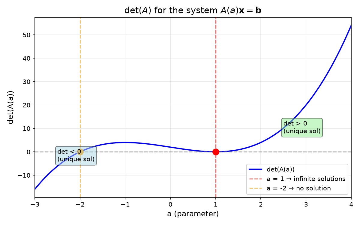The determinant crosses zero twice — at a = -2 and a = 1. Those are the critical values. Everywhere else, A is invertible and you get exactly one solution. At those two points something breaks; what happens depends on whether the RHS vector b lives in the column space of A.
Here’s the full script:
import numpy as np


def build_system(a):
    A = np.array([
        [a, 1, 1],
        [1, a, 1],
        [1, 1, a]
    ], dtype=float)
    b = np.array([6.0, 6.0, 6.0])
    return A, b

# Part 1: scan det(A) across values of a
a_values = np.linspace(-3, 4, 29)
dets = [np.linalg.det(build_system(a)[0]) for a in a_values]

for a, d in zip(a_values, dets):
    marker = " <-- SINGULAR" if abs(d) < 1e-9 else ""
    print(f"{a:6.2f} | {d:12.4f}{marker}")

# Part 2: case analysis at key values
for label, a in [
    ("unique: a=3", 3),
    ("unique: a=0", 0),
    ("singular: a=-2", -2),
    ("singular: a=1", 1),
]:
    A, b = build_system(a)
    det_val = np.linalg.det(A)
    rank_A = np.linalg.matrix_rank(A)
    rank_aug = np.linalg.matrix_rank(np.column_stack([A, b]))
    print(f"\na={a}: det={det_val:.4f}, rank(A)={rank_A}, rank([A|b])={rank_aug}")
    if abs(det_val) > 1e-9:
        x = np.linalg.solve(A, b)
        print(f"  -> UNIQUE: x={x.tolist()}")
    elif rank_A == rank_aug:
        free = A.shape[1] - rank_A
        print(f"  -> INFINITE (rank {rank_A}, {free} free var(s))")
    else:
        print(f"  -> NO SOLUTION (ranks differ)")
Running it
Here’s what Part 1 prints when we scan from a = -3 to a = 4:
a         |       det(A)
-------------------------
 -3.00 |     -16.0000
 -2.75 |     -10.5469
 -2.50 |      -6.1250
 -2.25 |      -2.6406
 -2.00 |       0.0000 <-- SINGULAR
 -1.75 |       1.8906
...
  1.00 |       0.0000 <-- SINGULAR
  1.25 |       0.2031
...
<video controls src="https://datmt-blog-media.datmt.com/uploads/source-material-is-python-book-all/out-febdefda-9526-4f52-a065-c0949a003587.mp4"></video>
Two important details are hiding in that scan. First, det(A) stays nonzero just before and after each zero — the matrix doesn’t “get close” to singular for nearby values, it is exactly singular only at those two points. Second, det = 0 doesn’t tell you which failure mode you’re in.
Looking at the four cases from Part 2 of the script:
a = 3 (unique): The solution is x = [1.2, 1.2, 1.2], with residual norm exactly 0.00e+00. Symmetry makes sense — every equation has identical structure, so every variable takes the same value.
a = 0 (unique): det(A) = 2 and x = [3.0, 3.0, 3.0]. This is a different point in parameter space with a completely different solution vector, but the behavior is the same — exactly one point satisfies all three equations.
a = -2 (no solution): det(A) = 0 and rank(A) = 2, but rank([A|b]) = 3. The coefficient matrix loses one degree of freedom, yet b pushes in a direction that none of the remaining columns can reach. This is an inconsistent system — no point exists that satisfies all three equations simultaneously.
a = 1 (infinite solutions): det(A) = 0 and rank(A) = rank([A|b]) = 1. The matrix collapses to a single independent equation (x + y + z = 6), so the solution is a whole plane in R^3 — any point on that plane works.
The verification section of the script confirms this last case: all four test points, including one with a negative coordinate (10, -4, 0), satisfy A * x = b when a = 1. Not every singular matrix produces infinite solutions; it only happens when b falls inside the column space.
Takeaway
A nonzero determinant guarantees exactly one solution and nothing else — that’s the easy half. When det(A) = 0, compare the rank of A to the rank of the augmented matrix [A|b]: equal ranks mean infinite solutions, unequal ranks mean no solution at all. The determinant tells you whether a unique solution exists; rank comparison tells you what happens next.