Applying Amdahl's Law Conceptually to Predict Scaling Ceilings
Amdahl’s Law is often presented as a formula students memorize for exams. Its practical value for developers isn’t in plugging numbers into the equation—it’s in asking one question about any system: what portion of this work fundamentally cannot be parallelized, even in principle?
The answer determines your scaling ceiling regardless of how many cores or nodes you throw at the problem. You can estimate it from code structure alone—no profiling required.
The code
Given a fraction P of work that is parallelizable and (1-P) that is serial, the maximum speedup across N processors is:
speedup = 1 / ((1 - P) + P/N)As N grows toward infinity, the speedup converges to 1 / (1 - P)—the serial fraction becomes the ceiling. This isn’t a property of your hardware; it’s a structural constraint baked into the problem itself.
The code below computes this across five parallel fractions and several processor counts, so you can see how the scaling curve bends:
# Compute Amdahl speedup for various parallel fractions
for P in [0.5, 0.8, 0.9, 0.95, 0.99]:
    serial = 1.0 - P
    limit = 1.0 / serial

    speedups = {}
    for N in [4, 8, 16, 32, 64, 128]:
        sp = 1.0 / (serial + P/N)
        speedups[N] = round(sp, 2)

    print(f"P={P:.2f} | ceiling: {limit:.1f}x")
    for N, sp in speedups.items():
        print(f"    N={N:>3d}: {sp:.2f}x")
    print()
Running it
The pattern is unmistakable. With P = 0.8 (just a 20% serial fraction), the ceiling is only 5.0x—no matter how many processors you add. Even at 128 processors, you’re still climbing toward that limit rather than approaching something close to 128x.
The P = 0.99 row (only 1% serial) looks impressive: it reaches 72x at 256 processors. But the asymptotic column reveals the true constraint—its ceiling is only 100x. At small scales everything looks fine; that tiny serial fraction doesn’t bite until you’re operating at scale.
Breaking down a real service
A typical service processes requests through several components. Some are naturally parallel (database queries on different rows), but others must execute in sequence:
work_breakdown = [
    ("Database queries", 0.55, "True parallelism"),
    ("Request routing", 0.10, "O(N) per request"),
    ("Session state serialization", 0.08, "Must be serialized"),
    ("Background job processing", 0.20, "Parallelizable with workers"),
    ("Cache warming (sequential I/O)", 0.05, "Disk-bound, sequential"),
    ("Metrics collection", 0.02, "Tiny but on critical path"),
]

# Identify what is inherently serial
serial_total = 0.13  # session serialization (8%) + cache warming (5%)
P_estimated = 1.0 - serial_total  # 0.87
Running this produces a ceiling of 7.7x:
| Processors | Speedup |
|---|---|
| 4 | 2.88x |
| 16 | 5.42x |
| 64 | 6.96x |
| 128 | 7.31x |
Between 16 and 128 processors—adding eight times the compute—the speedup only increases from 5.42x to 7.31x. The serial fraction has already claimed its share.
What if we fix the bottleneck?
Amdahl’s Law becomes actionable when you realize that fixing any serial portion shifts your entire curve upward:
scenarios = [
    (0.13, "Original"),      # serial fraction stays at 0.13
    (0.05, "Optimized"),     # eliminated session serialization
]

for serial_frac, label in scenarios:
    P_val = 1.0 - serial_frac
    print(f"Scenario {label} (serial={serial_frac:.2f}):")
    for N in [16, 64, 256]:
        sp = round(1.0 / (serial_frac + P_val/N), 2)
        print(f"  At {N:3d} processors: {sp:.2f}x speedup")
    print()
The session serialization component was only 8% of total work—yet it alone capped your ceiling at 7.7x. Eliminating it (replacing session state with distributed cache lookups, for instance) nearly doubles the speedup at scale (from 7.50x to 18.62x at 256 processors), even though you touched no parallel work whatsoever.
This is the structural insight: small serial fractions dominate your scaling budget. You can identify candidates for optimization by looking at data flow—where threads must synchronize, where state must be serialized, where I/O is inherently sequential—and treat those portions as a tax on every node you add.
Takeaway
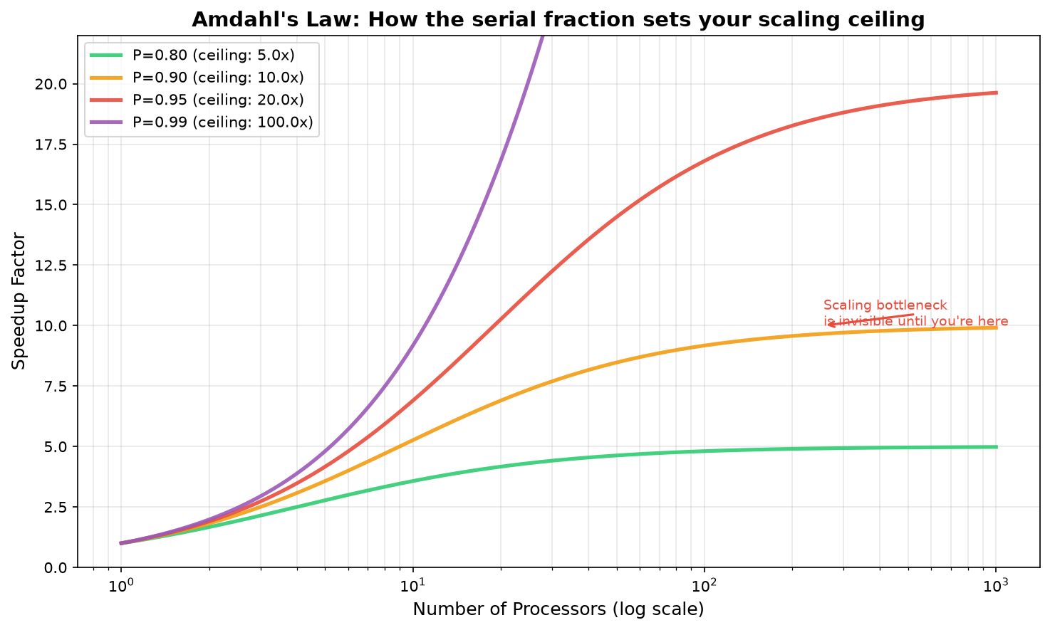
The plot above makes this geometrically obvious. Each curve flattens toward its asymptotic ceiling—the green line (P = 0.8) caps at 5x long before the purple line (P = 0.99) approaches 100x. The serial fraction doesn’t just reduce your speedup; it determines the shape of every intermediate step between single-core and infinite-scale.
At small processor counts, all curves look similar—they’re dominated by the parallel portion. At high counts, the divergence is dramatic. This is why scaling problems are invisible until you’re trying to operate at scale: everything looks fine until the serial fraction becomes the bottleneck.
Amdahl’s Law isn’t a calculation you perform once. It’s a mental filter: before adding parallelism, identify what portion of your system cannot be parallelized and let that number tell you whether more nodes are worth it. If the ceiling is too low for your goals, no amount of scaling will fix it—only redesigning those serial portions will.